
When we started building Bluefield's solar forecast models for western Japan sites, the first problem we encountered was not the model architecture. It was the data. And not in the way most ML practitioners mean when they say "data quality." The specific issues were resolution mismatches, systematic sensor gaps at the most operationally difficult periods, and a seasonal coverage structure that made the training set look comprehensive while hiding significant blind spots.
What follows is a description of the data properties that actually determine whether a solar forecast model will perform well at grid-dispatch resolution. It is grounded in what we have learned working with irradiance and generation records from Kyushu and Shikoku sites.
Resolution: Why 1-Hour Data Is Not Enough
Hourly irradiance data, from Japan Meteorological Agency surface observation stations or satellite-derived products, is sufficient for energy planning purposes. It is not sufficient for a dispatch-grade forecast model that needs to support 30-minute settlement interval decisions.
The problem is cloud transients. A cloud front moving through a solar field at midday can drop irradiance from 900 W/m2 to under 200 W/m2 in under 10 minutes, then recover. If your training data only has one irradiance value per hour, that event appears as a smooth partial-cloud hour. The model learns to treat similar weather patterns as gradual ramps. When deployed against 30-minute settlement intervals, it systematically underestimates the speed and depth of intra-hour drops.
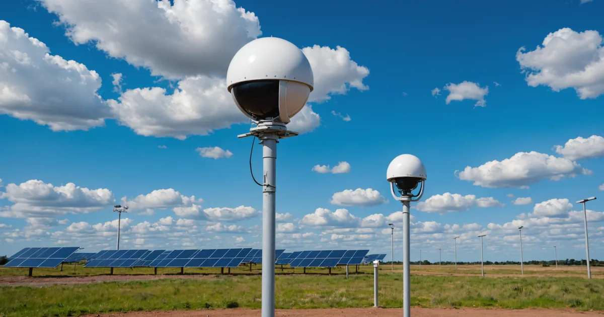
Training data for a dispatch-grade model should be at 10-minute or finer resolution, ideally from a pyranometer co-located with the generation asset or from a dense satellite-derived gridded product with sub-hourly timestamps. The JMA AMeDAS network provides 10-minute data at its surface observation stations, though the spatial coverage is uneven and the nearest station may be several kilometers from the target site with different terrain and microclimate characteristics.
When training data resolution cannot be improved, the model should incorporate an explicit uncertainty representation that widens the prediction interval for time steps following transitions in cloud cover. This is preferable to training against smooth hourly data and letting the model develop false confidence about intra-hour stability.
Gap Patterns: When Sensor Outages Are Not Random
Every irradiance dataset has gaps. Sensor maintenance, data logger failures, and communication outages create missing periods. The standard approach is imputation: fill gaps with a nearby station, with a satellite-derived estimate, or with a clear-sky model scaled to the recent observed bias. For training purposes, this is generally acceptable if the gaps are small and randomly distributed.
The problem appears when outages are systematic, meaning they cluster at specific conditions. In practice, sensor outages correlate with bad weather, because maintenance is deferred during wet periods, and with extreme events, because sensors can be damaged in high wind or heavy rain. This means a dataset with gaps is not missing a random sample of weather states. It is disproportionately missing records from the hardest-to-forecast conditions.
A model trained on such a dataset will underperform precisely on the days when accurate forecasting matters most. The training set is biased toward clear and partially-cloudy days where irradiance is predictable; the difficult overcast and storm-transition days are underrepresented.
The correct check is to tabulate gap frequency by weather type (using cloud cover classification from a reanalysis product or nearby station) and verify that gaps are not concentrated in the overcast category. If they are, the imputation method needs careful attention, or the model needs explicit treatment for these conditions using whatever data can be sourced for those periods.
Seasonal Coverage and the Rainy Season Gap
Japan's solar irradiance regime has strong seasonal structure. The tsuyu rainy season, typically running through June and into mid-July, produces extended overcast and highly variable irradiance patterns. The typhoon season from late summer through autumn brings a different volatility pattern. Winter months in western Honshu bring periodic heavy cloud cover from Sea of Japan weather systems.
A training dataset built from 18 months of records may look adequate on paper but has covered each of these regimes only once or not at all. A model trained with a single rainy season in the training set will have seen too few examples of tsuyu-type irradiance behavior to generalize well when the next June arrives.
The practical minimum for a deployment-ready model for a western Japan site is three full years of training data, covering at least three tsuyu seasons and three typhoon seasons. This is not an arbitrary threshold. It reflects the minimum sample size needed for the model to have seen enough examples of each distinct weather regime to learn regime-specific error patterns rather than collapsing to a single global error distribution.
We are not saying that two years of data is unusable. A model trained on two years will likely perform adequately in the four or five months of clear or winter weather, but its error distribution during tsuyu will be poorly constrained. If the operational use case includes market participation during June and July, the model needs the additional seasonal coverage.
Plant-Specific Generation Records vs. Irradiance Alone
Irradiance data captures the available solar resource. It does not capture what the plant actually does with that resource, which depends on inverter efficiency curves, clipping behavior at high irradiance, soiling effects, and partial shading from cloud patterns across a large panel array.
For dispatch-grade forecasting, the target variable is AC output in MW, not irradiance. The relationship between irradiance and AC output is not linear. At high irradiance, inverter clipping limits output. At low irradiance, inverter startup thresholds mean the plant is offline even when the irradiance is marginally positive. Soiling reduces effective irradiance non-uniformly across the array.
Training directly on plant generation records, alongside irradiance as a feature, captures these plant-specific characteristics in the model parameters rather than requiring the operator to specify them explicitly. This is particularly valuable for sites with older inverter equipment, partial shading geometries, or non-standard array configurations.
The requirement is at least two years of metered generation data at 10-minute or 30-minute resolution, quality-controlled for forced outages (which should be flagged in the training data so the model does not learn to treat curtailment as a weather-driven generation event).
The Data Pipeline Is Part of the Model
A final point that is often underweighted: the data pipeline that feeds new observations into the deployed model is as important as the training dataset. If the live forecast runs on different data sources than the training data, or if the preprocessing chain introduces lags or transformations that were not present during training, the model will operate outside the distribution it was trained on.
This is a concrete risk when training uses high-quality historical reanalysis data but deployment uses near-real-time NWP model output, which has different bias characteristics. The solution is to train the model on data that has been through the same preprocessing steps as the live operational pipeline, including any bias corrections and spatial interpolation methods applied to the NWP source. The training-deployment distribution gap is one of the more common sources of forecast model degradation that only becomes visible after the system goes live.